Word Embeddings Explained: From Word2Vec to BERT and Beyond

January 25, 2021

Embeddings visualised. Picture sourced from Bio-inspired Structure Identification in Language Embeddings

While computers are very good at crunching numbers and executing logical commands, they still struggle with the nuances of the human language! Word embeddings aim to bridge that gap by constructing dense vector representations of words that capture meaning and context, to be used in downstream tasks such as question-answering and sentiment analysis. The study of word embedding techniques forms part of the field of computational linguistics. In this article we explore the challenges of modelling languages, as well as the evolution of word embeddings, from Word2Vec to BERT.

Computational Linguistics

Prior to the recent renewed interest in neural networks, computational linguistics relied heavily on linguistic theory, hand-crafted rules, and count-based techniques. Today, the most advanced computational linguistic models are developed by combining large annotated corpora and deep learning models, often in the absence of linguistic theory and hand-crafted features. In this article, I aim to explain the fundamentals and different techniques of word embeddings, whilst keeping the jargon to a minimum and the calculus in the negative.

“What’s a corpus/corpora?” you may ask. Very good question. In linguistics, a corpus refers to an entire set of a particular linguistic element within a language, such as words or sentences. Typically, corpuses (or corpora), are monolingual (of a uniform language) collections of news articles, novels, movie dialogues, etc, etc.

Rare and unseen words

The frequency distribution of words in large corpuses follow something called Zipf’s Law. This law states that, given some corpus of natural language utterances, the frequency of any word is inversely proportional to their rank. This means that if a word like “the” has rank 1 (meaning its the most frequent word), its relative frequency to the rest of the corpus is 1. And, if a word like “of” has rank 2, its relative frequency would be 1/2. And so forth.

Sourced from https://www.smashingmagazine.com/2012/05/stop redesigning-start-tuning-your-site/

The implications of Zipf’s law is that a word with rank 1000 would occur once for every 1st rank word like “the”. And it gets even worse as your vocabulary grows! Zipf’s law means that some words are so rare that they might occur only a few times in your training data of several thousand pieces of text. Or worse, the rare words are absent in your training data but present in your testing data, also known as out-of-vocabulary (OOV) words. This means that researchers need to employ different strategies to upsample the infrequently-found words (also called the long tail of the distribution) as well as build models that are robust to unseen words. Some strategies to deal with these challenges include upsampling, using n-gram embeddings (like FastText) and character-level embeddings, such as ElMo.

Word2Vec, the OG

Every person that has tried their hand at NLP is probably familiar with Word2Vec, which was introduced by Google researchers in 2013. Word2Vec consists of two distinct architectures: Continuous Bag-of-Words (or CBOW) and Skip-gram. Both models produce a word embedding space where similar words are found together, but there is a slight difference in their architectures and training techniques.

Sourced from https://arxiv.org/pdf/1309.4168v1.pdf

With CBOW, we train the model by trying to predict a target word w given a context vector. Skip-gram is the inverse; we train the model by trying to predict the context vector given the target word w. The context vector is just a bag-of-words representation of the words found in the immediate surroundings of our target word w, as shown in the graphic above. Skip-gram is more computationally expensive than CBOW, so down-sampling of distant words is applied to give them less weight. To address the imbalance between rare and common words, the authors also aggressively sub-sampled the corpus — with the probability of discarding a word being proportional to its frequency.

Sourced from https://developers.google.com/machine-learning/crash-course/embeddings/translating-to-a-lower-dimensional-space

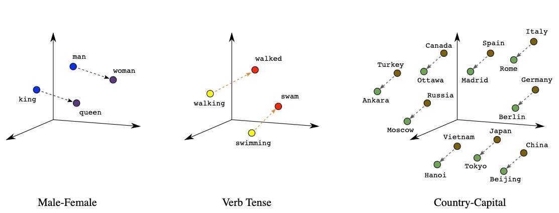
The researchers also demonstrated the remarkable compositionality property of Word2Vec, such that one can perform vector addition and subtraction with word embeddings and find “king” + “women” = “queen”. Word2Vec opened the door to the world of word embeddings, and sparked a decade where language processing now needed bigger and badder machines, and relied less and less on linguistic knowledge.

FastText

The embedding techniques we have discussed up until now represent each word of the vocabulary with a distinct vector, thus ignoring the internal structure of words. FastText extends the Skip-gram model by also taking into account subword information. This model is ideal for languages where grammatical relations like Subject, Predicate, Objects, etc., are reflected by inflections — words are morphed to express changes in their meanings or grammatical relations, rather than by the relative positions of the words or by adding particles.

The reason for this is that FastText learns vectors for character n-grams (almost like subwords — we will get to that in a moment). Words are then represented as the sum of the vectors of their n-grams. The subwords are created as follows:

• each word is broken up into a set of character n-grams, with special boundary symbols at the beginning and end of each word,

• the original word is also retained in the set,

• for example, for n-grams of size 3 and the word “there”, we have the following n-grams:

<th, the, her, ere, re> and the special feature <there>.

There is a clear distinction between the features <the> and the. This simple approach enables sharing representations across the vocabulary, can handle rare words better, and can even handle unseen words (a property the previous models lacked). It trains fast and requires no preprocessing of the words nor any prior knowledge of the language. The authors performed a qualitative analysis and showed that their technique outperforms models that do not take subword information into account.

ELMo

ELMo is an NLP framework developed by AllenNLP in 2018. It constructs deep, contextualized word embeddings that can deal with unseen words, syntax and semantics, as well as polysemy (words taking on multiple meanings given the context). ELMo makes use of a pre-trained two-layer bi-directional LSTM model. The word vectors are extracted from the internal states of a pre-trained deep bidirectional LSTM model. Instead of learning representations for word-level tokens, ELMo is trained to learn representations for character-level tokens. This allows it to effectively deal with out-of-vocabulary words during testing and inference.

The inner workings of a biLSTM. Sourced from https://www.analyticsvidhya.com/

The architecture consists of two layers stacked together. Each layer has 2 passes — a forward pass and a backward pass. To construct character embeddings, ELMo employs character-level convolutions over the input words. The forward pass encodes the context of the sentence leading up to and including a certain word. The backward pass encodes the context of the sentence after and including that same word. The combination of forward and backward LSTM hidden vector representations are concatenated and fed into the second layer of the biLSTM. The final representation (ELMo) is the weighted sum of the raw word vectors and the concatenated forward and backward LSTM hidden vector representations of the second layer of the biLSTM.

What made ELMo so revolutionary at that time (yes, 2018 was a long time ago in NLP years) is that each word embedding encoded the context of the sentence, and that word embeddings were functions of their characters. Thus, ELMo simultaneously addressed the challenges posed by polysemy and unseen words. Besides English, pre-trained ELMo word embeddings are available in Portuguese, Japanese, German, and Basque. The pretrained word embeddings can be used as is in downstream tasks, or further tuned on domain-specific data.

BERT

Google Brain researchers introduced BERT in 2018, a few months after ELMo. Back then, it smashed records for 11 benchmark NLP tasks, including the GLUE task set (which consists of 9 tasks), SQuAD, and SWAG. (Yes, the names are funky, NLP is full of really fun people!)

Sourced from https://syncedreview.com/2020/03/13/bertlang-helps-researchers-choose-between-bert-models/

BERT stands for Bidirectional Encoder Representations from Transformers. Unsurprisingly, BERT makes use of the encoder part of the Transformer architecture, and is pre-trained once in a pseudo-supervised fashion (more on that later) on the unlabelled BooksCorpus (800M words) and the unlabelled English Wikipedia (2,500M words). The pre-trained BERT can then be fine-tuned by adding an additional output (classification) layer for use in various NLP tasks.

If you are unfamiliar with the Transformer (and Attention Mechanisms), check out this article I wrote on the topic. In their highly-memorable paper titled “Attention Is All You Need”, Google Brain researchers introduced the Transformer, a new type of encoder-decoder model that relies solely on attention to draw global dependencies between the input and output sequences. The model injects information about relative and absolute positions of tokens using positional encodings. A token representation is calculated as the sum of the token embedding, the segment embedding and the positional encoding.

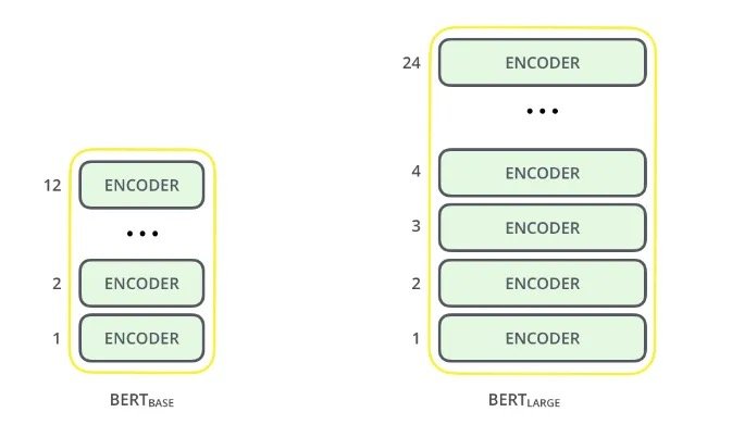
In essence, BERT consists of stacked Transformer encoder layers. In Google Brain’s paper, they introduce two variants: BERT Base and BERT Large. The former consists of 12 encoder layers and the latter 24. Similar to ELMo, BERT processes sequences bidirectionally, which enables the model to capture context from left to right, and then again from right to left. Each encoder layer applies self-attention, and passes its outputs through a feed-forward network, and then onto the next encoder.

Alammar, J (2018). The Illustrated Transformer [Blog post]. Retrieved from https://jalammar.github.io/illustrated-transformer/

BERT is pretrained in a pseudo-supervised fashion using two tasks:

• Masked Language Modelling

• Next Sentence Prediction

Why I say pseudo-supervised is because neural networks inherently need supervision to learn. To train the Transformer, we transform our unsupervised tasks into supervised tasks. We can do this with text, which may be considered series of words. Remember that the term bidirectionalmeans that the context of a word is a function of the words preceding it and by the words following it. Self-attention combined with bidirectional processing would mean that the language model is all-seeing, making it difficult to actually learn the latent variables. Along comes Masked Language Modelling, which exploits the sequential nature of text, and makes the assumption that a word can be predicted using the words surround it (the context). For this training task, 15% of all the words are masked.

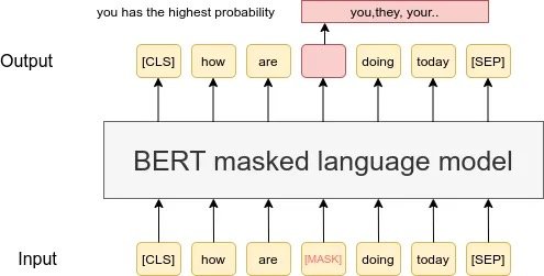
Sourced from researchgate.net

The MLM task helps the model learn the relationships between different words. The Next Sentence Prediction (NSP) task helps the model learn the relationships between different sentences. NSP is structured as a binary classification task: given Sentence A and Sentence B, does B follow A, or is it just a random sentence?

These two training tasks are enough to learn really complex language structures — in fact, a paper titled “What does BERT learn about the structure of language?” demonstrated how the layers of BERT captures more and more granular levels of language syntax. The authors showed that the bottom layers of BERT capture phrase-level information, while the middle layers capture syntactic information, and the top layers semantic information.

Since its inception, BERT has inspired many recent state-of-the-art NLP architectures, training approaches and language models, including Google’s TransformerXL, OpenAI’s GPT-3, XLNet, RoBERTa, and Multilingual BERT. It’s universal approach to language understanding means that it can be fine-tuned with minimal effort to a variety of NLP tasks, including question-answering, sentiment analysis, sentence-pair classification, and named entity recognition.

Conclusion

While word embeddings are very useful and easy to compile from a corpus of texts, they are not magic unicorns. We highlighted the fact that many word embeddings struggle with disambiguity and out-of-vocabulary words. And although it is relatively easy to infer semantic relatedness between words based on proximity, it is much more challenging to derive specific relationship types based on word embedding. For example, even though puppy and dog may be found close together, knowing that a puppy is a juvenile dog is much more challenging. Word embeddings have also been shown to reflect ethnic and gender biases that are present in the texts that they are trained on.

Word embeddings are truly remarkable in their ability to learn very complex language structures when trained on large amounts of data. To the untrained eye (or untrained 4IR manager), it may even seem magical, and therefore it is very important to highlight and keep these limitations in mind when we use word embeddings.

If you enjoyed this blog post, please consider supporting my writing by buying me a coffee.

Transformers: Age of Attention

November 26, 2020

In their highly-memorable paper titled “Attention Is All You Need”, Google Brain researchers introduced the Transformer, a new type of encoder-decoder model that relies solely on attention for sequence-to-sequence modelling. Before the Transformer, attention was used to help improve the performance of the likes of Recurrent Neural Networks (RNNs) on sequential data.

Now, this is a lot. You might be wondering, “What the hell is sequence-to-sequence modelling, Jeanne?” You may also suffer from an attention deficiency, so allow me to introduce you to…

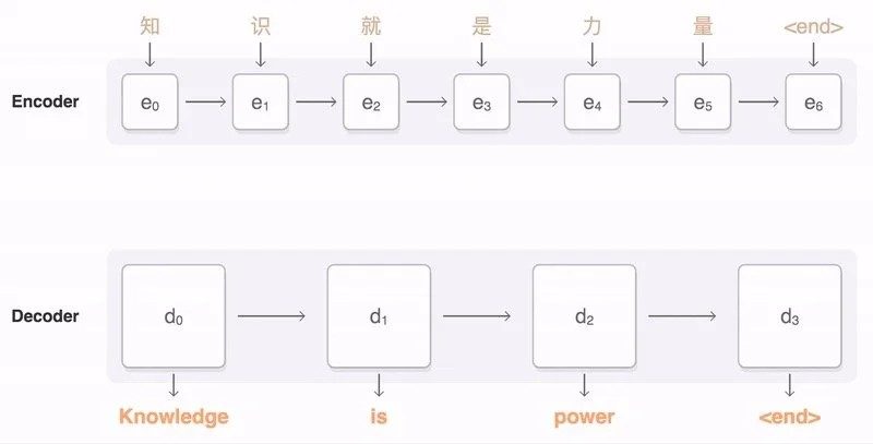
Seq2seq models

Sequence-to-sequence models (or seq2seq, for shorthand) are a class of machine learning models that translates an input sequence to an output sequence. Typically, seq2seq models consist of two distinct components: an encoder and a decoder. The encoder constructs a fixed-length latent vector(or context vector) of the input sequence. The decoder uses the latent vector to (re)construct the output or target sequence. Both the input and output sequence can be of variable length.

The applications of seq2seq models extend beyond simply machine translation. The architecture of the encoder-decoder model can be used for question-answering, mapping speech-to-text and vice versa, text summarisation, image captioning, as well as learning contextualised word embeddings.

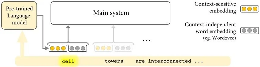
Unlike (context-independent) word embeddings, which have static representations, contextualized embeddings have dynamic representations that are sensitive to their context. Sourced from Researchgate

The novel RNN Encoder-Decoder model was introduced in 2014 by renowned researcher Kyunghyun Cho and his team, to perform statistical machine translation. This model uses the final hidden representations of the encoder RNN as context vector for the decoder RNN. This approach works fine for short sequences, but fails to accurately encode longer sequences. In addition, RNNs suffer from Vanishing Gradients, and are slow to train. Adding the attention mechanism to the RNN encoder-decoder architecture helps improve on its ability to model long-term dependencies.

Attention? Attention!

Attention is a function of the hidden states of the encoder to help the decoder decide which parts of the input sequence are most important for generating the next output token. Attention allows the decoder to focus on different parts of the input sequence at every step of the output sequence generation. This means that dependencies can be identified and modeled, regardless of their distance in the sequences.

Attention applied to an input sequence to assist in machine translation

When attention is added to the RNN encoder-decoder, all the encoder’s hidden representations are used during the decoding process. The attention mechanism creates a unique mapping between the output of the decoder and the hidden states of the encoder at each time step. These mappings reflects how important that part of the input is for generating the next output token .Thus, the decoder can “see” the entire input sequence and decide which elements to pay attention to when generating the next output token.

There are two major types of attentions: Bahdanau Attention, and Luong Attention.

Bahdanau Attention works by aligning the decoder with the relevant input sentences. The alignment scores is a function of the hidden states produced by the decoder in the previous time step and the encoder outputs. The attention weights are the output of softmax applied to the alignment scores. After this, the encoder’s outputs and their attention weights are multiplied element-wise to form the context vector.

The context vector of Luong Attention is calculated similarly to Bahdanau’s Attention. The key differences between the two are as follows:

• with Luong Attention, the context vector is only utilized after the RNN produced the output for that time step,

• the ways in which the alignment scores are calculated, and

• the context vector is concatenated with the decoder hidden state to produce a new output.

There are three different ways to compute the alignment scores: dot-product (multiply the hidden states of the encoder and decoder), general (multiply the hidden states of the encoder and decoder, preceded by a multiplication with a weight matrix), and concatenation (a function applied on top of adding together the hidden states of the encoder and decoder). More information on this can be found here. Subsequently, the context vector, together with the previous output will determine the new hidden state of the decoder.

The Transformer

Google Brain researchers flipped the tables on the NLP community and showed that sequential modelling can be done using just attention, in their 2017 paper titled “Attention is all you need”. In this paper, they introduce the Transformer, a simplistic architecture that makes use of only attention mechanisms to draw global dependencies between input and output sequences.

The Transformer consists of two parts: an encoding component and a decoding component. Additionally, positional encodings are injected to give information about the absolute and relative positions of the tokens.

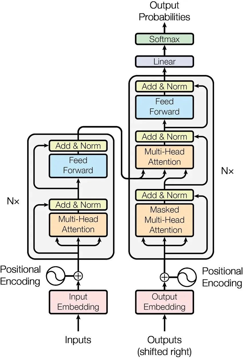
The Encoder-Decoder Model

Sourced from papers.nips.cc/paper/7181-attention-is-all-you-need.pdf

The encoding component is a stack of 6 encoders. Although identical, the encoders do not have shared weights. Each encoder can be deconstructed into a multi-head attention part and a fully connected feed-forward network.

Similarly, the decoding component is a stack of 6 identical decoders, whose architecture is similar to the encoder’s, except it masks its multi-head attention to ensure that the next output can only depend on the known outputs of the previous tokens. Also, the decoder has an extra multi-head attention component that applies self-attention over the output of the encoding component, providing access to the inputs during decoding.

Multi-head attention

Each multi-head attention component consists of several attention layers running in parallel. The Transformer makes use of scaled dot-product attention, which is very similar to Luong’s dot-product attention, except it is scaled. Multi-headed attention allows for scaled dot-product attention to be aggregated across n different, randomly-initialized representation subspaces. This multi-headed attention function can also be parallelized and trained across multiple computers.

Why Transformers?

Much like Recurrent Neural Networks (RNNs), Transformers allows for processing sequential information, but in a much more efficient manner. The Transformer outperform RNNs, both in terms of accuracy and computational efficiency. Its architecture is devoid of any recurrence or convolutions, and thus training can be parallelizable across multiple processing units. It has achieved state-of-the-art performance on several tasks, and, even more importantly, was found to generalize very well to other NLP tasks, even with limited data.

In conclusion

The Transformer has taken the NLP community by storm, earning a place among the ranks of Word2Vec and LSTMs. Today, some of the state-of-the-art language models are based on the Transformer architecture, such as BERTand GPT-3. In this blog post, we discussed the evolution of sequence-to-sequence modelling, from RNNs, to RNNs with Attention, to solely relying on attention to model input to output sequences with the Transformer.

If you enjoyed this blog post, please consider supporting my writing by buying me a coffee.